cat though, he was just along for the ride.
|
|
|
|
cat though, he was just along for the ride. |
|
I am a mathematical biologist who has researched at the oldest and newest universities in the United States ( Harvard and UC Merced ). This web page summarizes some of the more notable themes of my work.
|
|
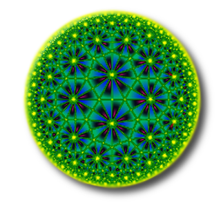
Symmetry is an important concept for understanding many of the patterns found in Nature. The presence of some type of repetition is an essential feature of symmetry. Sometimes the repetition takes on a precise geometric form but more often there are minor differences between the repeated portions of a pattern. The figure above on the right has a checkerboard like pattern but, in terms of Euclidean geometry, only a few of the squarish regions are congruent to one another. For the most part the squarish regions have different Euclidean shapes even though they fit neatly together to create the symmetrical pattern.
|
|
 Stamens on the Australian flower Leucadendron Discolor
|
Phyllotaxis is the scientific name for how body parts are arranged on plants. Phyllotaxis provides interesting examples of symmetry in biology because the same types of patterns are formed by many different types of plant organs. A common eye catching pattern resembles a lattice made up of two sets of spiral shaped curves. A few examples shown on this web page are flower stamens, cactus thorns, succulent leaves, and the florets of compound flowers. |
 Thorns on a prickly pear cactus
|
Around the beginning of the 1700's the well known astronomer Johanne Kepler pointed out that the Fibonacci numbers are common in plants. The Fibonacci numbers form a sequence in which each member is the sum of the previous two members. The sequence begins with 1 and 1. Since 1+1=2 the next Fibonacci number is 2. The Fibonacci sequence goes |
|
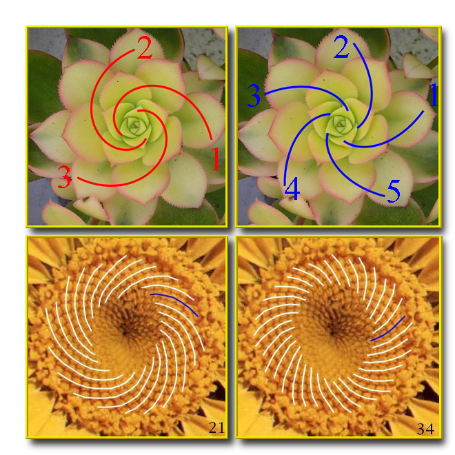
Around 1790 the botanist Charles Bonnet elaborated on Kepler's observation. Bonnet explained that for many of the spiral patterns found in plants the number of spirals coiling outward in the clockwise and counter-clockwise directions are two successive Fibonacci numbers. For example in the succulent plant shown below the number of spirals coiling outward in the clockwise direction is 3 and the number of spirals coiling outward in the counter-clockwise direction is 5. |
|
|
In phyllotaxis these spirals are called parastichies. Paradoxically the parastichies are easier to see when the numbers are bigger. The leaves of the succulent are far apart so we have to look carefully to see how they are arranged into parastichies. The florets in the daisy shown above are packed tightly together and it is easier to see the parastichies. The number of parastichies coiling outward in the clockwise direction is 21 and the number of parastichies coiling outward in the counter-clockwise direction is 34. The number of parastichies coiling clockwise and counter-clockwise are called the parastichy numbers of the phyllotactic pattern. An intriguing feature of phyllotaxis can be concisely stated as What is even more intriguing about phyllotaxis is that Lucas numbers are like Fibonacci numbers in that they form a sequence in which each member is the sum of the previous two members. But for Lucas numbers the sequence begins with 1 and 3. Since 1+3=4 the next Lucas number is 4. The Lucas sequence goes Understanding why consecutive Fibonacci numbers and, to a lessor extent, consecutive Lucas numbers are common throughout much of the plant kingdom has become an interdisciplinary effort. Several ideas have been proposed over the years many of which have been based on the notion that the Fibonacci numbers somehow promote the survival of mature plants. Among the suggestions on how Fibonacci (or Lucas) numbers could promote survival are: by providing dense packings of seeds, by allowing circulation of air through leaves, and by allowing light to fall on as many leaves as possible. A more modern view is that a common physicochemical condition occurs in the early stages of development that constrains plant tissue to follow certain developmental pathways. The significance of the Fibonacci numbers does not lie in some activity performed by a mature plant but in the activity that occurs while the plant organs are forming. The Fibonacci numbers are not seen as doing very much to promote or hinder survival in mature plants. A daisy whose flowers have 20 parastichies coiling in one direction and 35 parastichies coiling in the opposite direction should produce about same number of viable seeds for the next generation as a daisy whose flowers have 21 parastichies coiling in one direction and 34 parastichies coiling in the opposite direction. Yet the first case is virtually unheard of while the second case is very common. You can learn more at the links |
|
 |
Symmetry is often thought of as a purely geometric phenomenon and it is usually defined in terms of rigid motions of a figure to itself but there are other types of symmetry. Rather than get into all of the technicalities I will explain the concept of topological symmetry by looking at three examples. In these examples we will only consider a finite number of topological symmetries. In an Euclidean plane this restriction provides a strong constraint on the types of symmetry that can occur but in higher dimensions this restriction is not so strong and it allows for some rather exotic types of topological symmetry to occur.
|
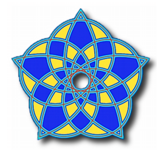
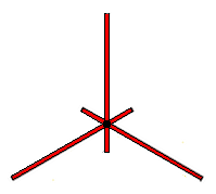
Our first example of topological symmetry is shown in the diagram on the left. It depicts a geometric figure made up of six line segments connected at a single point in the center. Geometrically speaking the figure has the same type of symmetry as an equilateral triangle. Like an equilateral triangle we can rotate the figure by one third of a turn, two thirds of a turn, and we can reflect it about three different lines in the plane. When we include the identity map we get six Euclidean symmetries altogether, but there are more symmetries hidden in this figure.
The intrinsic structure of the figure provides one kind of constraint on how it can be mapped to itself. The vertex in the center must be mapped to itself and each line segment must either be mapped to itself or to some other line segment. The fact that the figure is embedded in the plane provides another kind of constraint. The cyclic order of the line segments radiating away from the central vertex must either be preserved or reversed.
A consequence of restricting ourselves to finite groups of topological symmetries introduces another more subtle constraint. A transformation which maps a line segment to itself must map every point in the line segment to itself. Otherwise repeatedly applying the transformation would generate an infinite number of transformations. Therefore any transformation which maps all six line segments to themselves must fix every point of the figure.
There are six ways we can map the six line segments so that their cyclic order is preserved and six ways we can map them so their cyclic order is reversed. If two transformations permuted the line segments in the same way then combining either of these transformations with the inverse of the other would produce a transformation that maps every line segment back to itself and therefore must fix every point of the figure. This implies that the two transformations must actually be the same. So the only finite groups of transformations of the plane to itself that can be symmetries of the figure have at most twelve members.
These twelve symmetries are very much like the Euclidean symmetries found in a regular hexagon. Indeed if we stretched the three short line segments radially outward so that they had the same length as the three long line segments then the line segments would form the diagonals of a regular hexagon and the whole figure would have the Euclidean symmetry of a regular hexagon.
Even though this figure has more topological symmetries than Euclidean symmetries these topological symmetries did not give the figure a new type of symmetry. The topological symmetry is the same type as the Euclidean symmetry of a different figure. This is generally true in two dimensions. Figures in the Euclidean plane with a finite number of topological symmetries can be continuously deformed without changing their topology so that their topological symmetries become Euclidean symmetries given by rigid rotations and/or reflections of plane.
|
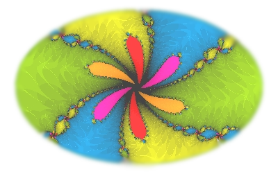
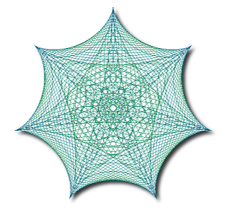
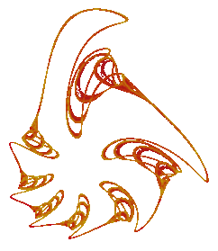
Our second example of topological symmetry is the fractal to the left which is the attractor for a discrete dynamical system obtained by numerically integrating the Volterra-Lotka equations . The Volterra-Lotka equations were one of the original mathematical models of predator/prey relationships and they are well known among population biologists. In this mathematical model the population sizes of the predator and prey species vary over time in a precisely periodic fashion. If we plot the population size of the prey versus the population size of the predator then over time these points will trace out a simple closed curve in the plane.
However in making this fractal the time step of the numerical method has been deliberately made too large for the purpose of approximating the solutions to the Volterra-Lotka equations. Making the time step too large in the numerical integration of a differential equation often results in a map that has a fractal attractor. This is a convenient way to custom design fractals.
To help understand how this works consider using a small time step in the numerical method and imagine slowly increasing its size. For small enough values of the time step most numerical methods do a good job of approximating the periodic solutions of the Volterra-Lotka equations. As the numerical method is iterated it produces a discrete set of points which tends to closely follow one of the simple closed curves for the Volterra-Lotka equations.
As the time step increases "resonances" can occur in the numerical method. In other words an attractor appears which consists of just a finite set of points. In this particular case the number of points in the attractor was seven. The numerical method mapped each point of the attractor to another point of the attractor and in every seven iterations each point of the attractor is visited. In this case we say that the periodicity of the resonance is seven. Many different starting values tend to converge towards the seven point attractor.
The periodicity of the resonances can be controlled by appropriately choosing the numerical method. In this case increasing the time step a little more resulted in a period doubling bifurcation. A pair of points emerged from each of the seven points in the original attractor. This produced a fourteen point attractor while the previous seven points formed a repellor. Further increasing the time step resulted an infinite sequence of period doubling bifurcations that produced a fractal attractor for the system.
This fractal can not be rotated or reflected back into itself. Aside from the identity map there is no rigid motion or congruence of the Euclidean plane which can map this fractal into itself. However the period seven resonance has effectively given us an attractor which can be decomposed into seven topologically equivalent pieces. These seven pieces emerged from the seven points of the original period seven resonance through the period doubling cascade. Each of these seven pieces individually resembles maple syrup being poured out from a bottle. Geometrically these pieces have different shapes but their complicated topological structures are the same. The numerical method maps each piece of this attractor to another piece of this attractor and in every seven iterations each of these pieces is visited.
Although the symmetry of this fractal is, in sense, hidden the type of symmetry that it displays is not really new. We can stretch and compress regions of the plane to turn this fractal into a figure which can be mapped back into itself with a rigid rotation by one seventh of a turn.
|
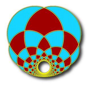
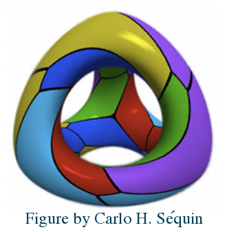
If we relax the requirement that the group of topological symmetries has to extend to a group of homeomorphisms of the entire Euclidean space then we can find many interesting examples of topological symmetry in three dimensions. Our third example is an object often referred to as "Klein's quartic surface" shown to the left. This is a highly symmetrical figure made up of twentyfour regular heptagons with three heptagons meeting at each vertex. It is like the five Platonic solids (regular polyhedra) but it has to be distorted to fit inside three dimensional Euclidean space, E3. Klein's quartic can be embedded in a higher dimensional space in which it is possible to rigidly rotate the figure by a seventh of a turn about the center of each heptagon. But in E3 these symmetries involve stretching and compressing different parts of the figure.
Altogether the group of topological symmetries for Klein's quartic has 336 members. It is very different from any geometric symmetry group in E3. For instance any polyhedron in E3 can have at most one axis in which it can be rotated by a seventh of a turn. But for each curved heptagon in an embedding of Klein's quartic in E3 there is a homeomorphism which maps the figure to itself, the chosen heptagon to itself, and the heptagon's edges to adjacent edges. The homeomorphism fixes exactly one point in the interior of the heptagon and on "average" the other points in the heptagon are rotated about the fixed point by one seventh of a turn. In this sense we can rotate the figure by one seventh of a turn about every one of its faces. These homeomorphisms can be extended to all of E3 except for a subset with zero volume.
The picture of Klein's quartic embedded in E3 is from "Patterns on the Genus-3 Klein Quartic" which has many other nice pictures of Klein's quartic. This article is available online. A whole book has been written on this object: "The Eightfold Way: The Beauty of Klein's Quartic". This book is also available online. Below is a list of links to these and other websites with pictures and text which explain the topological symmetry of Klein's quartic in greater detail.
You can learn more about fractals like the one above in the book
| "Chaos in Discrete Dynamical Systems" , by Ralph Abraham, Laura Gardini, and Christian Mira. |
Would you like to be able to visualize geometric figures in spaces with more than three dimensions? The link below is for an open source program which projects configurations of points in high dimensional Euclidean spaces into three dimensions. The projection methods includes principal component analysis and the Sammon map. The Sammon maps is useful when finite point sets are used to represent continuous media because it tends to respect the topology of the continuous media.
| The HiSee software website |